Build and train neural network models using TensorFlow 2.x▸
Time series, sequences and predictions▸
Natural language processing (NLP)▸
The goal of this certificate is to provide everyone in the world the opportunity to showcase their expertise in ML in an increasingly AI-driven global job market. This certificate in TensorFlow development is intended as a foundational certificate for students, developers, and data scientists who want to demonstrate practical machine learning skills through the building and training of models using TensorFlow.
The certificate program requires an understanding of building TensorFlow models using Computer Vision, Convolutional Neural Networks, Natural Language Processing, and real-world image data and strategies.
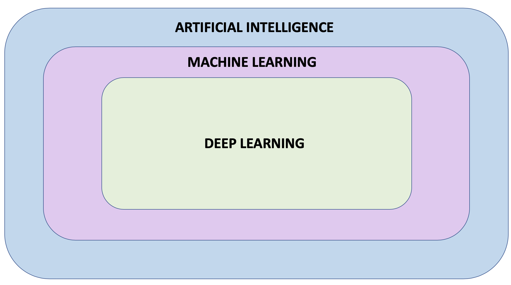
Artificial Intelligence: A field of computer science that aims to make computers achieve human-style intelligence. There are many approaches to reaching this goal, including machine learning and deep learning.
In supervised learning, the machine uses labeled training data. It is told the correct output and it compares its own output which informs the subsequent steps, adjusting itself along the way.
The Supervised Learning mainly divided into two parts:
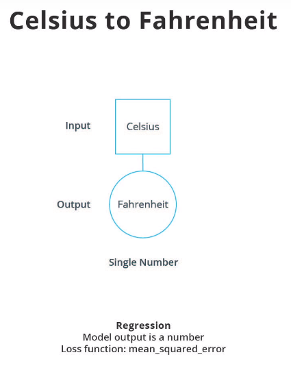
A machine learning model used to predict continuous value.
Regression algorithms - predict one or more continuous numeric variables.
Association algorithms - find correlations between different attributes in a dataset. The most common application of this kind of algorithm is for creating association rules, which can be used in a market basket analysis.
A machine learning model used for distinguishing among two or more output categories.
In unsupervised learning, the data isn't labeled. The machine must figure out the correct answer without being told and must therefore discover unknown patterns in the data.
Some popular examples of unsupervised learning include GANs and Autoencoders.
The Unsupervised Learning mainly divided into two parts:
Clustering is a Machine Learning technique that involves the grouping of data points. Given a set of data points, we can use a clustering algorithm to classify each data point into a specific group.
Machine Learning technique reduces the dimensionality of training data. The module analyzes input data and creates a reduced feature set that captures all the information contained in the dataset, but in a smaller number of features.
In Semi-Supervised Learning: Input data is a mixture of labeled and unlabeled examples.
Reinforcement Learning allows the machine the most freedom. It uses trial and error to discover the actions that yield the greatest rewards. AlphaGo is a famous example of RL.
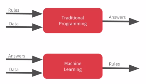
Traditional programming languages typically take data and rules as input
and apply the rules to the data in order to come up with answers as
output.
On the other hand, in machine learning paradigm the data and answers (or
labels) go in as input and the learned rules (models) come out as output.
Machine learning paradigm is uniquely valuable because it lets computer to
learn new rules in complex and high dimensional space, a space harder to
comprehend by humans.
The training process (happening in model.fit(...)) is really about tuning the internal variables of the networks to the best possible values, so that they can map the input to the output. This is achieved through an optimization process called Gradient Descent, which uses Numeric Analysis to find the best possible values to the internal variables of the model.
Gradient descent iteratively adjusts parameters, nudging them in the correct direction a bit at a time until they reach the best values. In this case “best values” means that nudging them any more would make the model perform worse.
The function that measures how good or bad the model is during each iteration is called the “loss function”, and the goal of each nudge is to “minimize the loss function.
The training process starts with a forward pass, where the input data is fed to the neural network (see Fig.1). Then the model applies its internal math on the input and internal variables to predict an answer ("Model Predicts a Value" in Fig. 1). In our example, the input was the degrees in Celsius, and the model predicted the corresponding degrees in Fahrenheit.
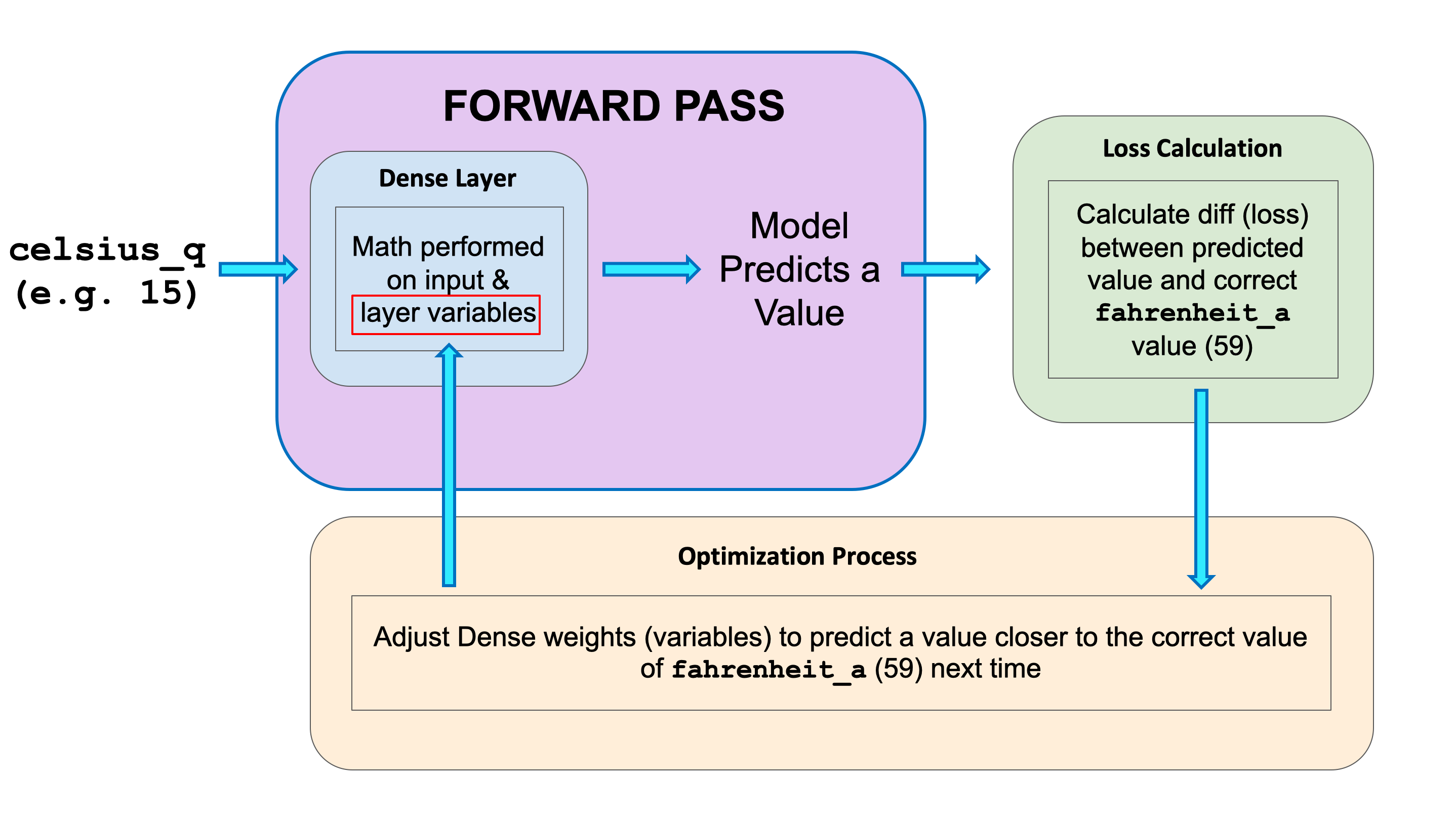
Once a value is predicted, the difference between that predicted value and the correct value is calculated. This difference is called the loss, and it's a measure of how well the model performed the mapping task. The value of the loss is calculated using a loss function, which we specified with the loss parameter when calling model.compile().
After the loss is calculated, the internal variables (weights and biases) of all the layers of the neural network are adjusted, so as to minimize this loss — that is, to make the output value closer to the correct value (see Fig. 2).
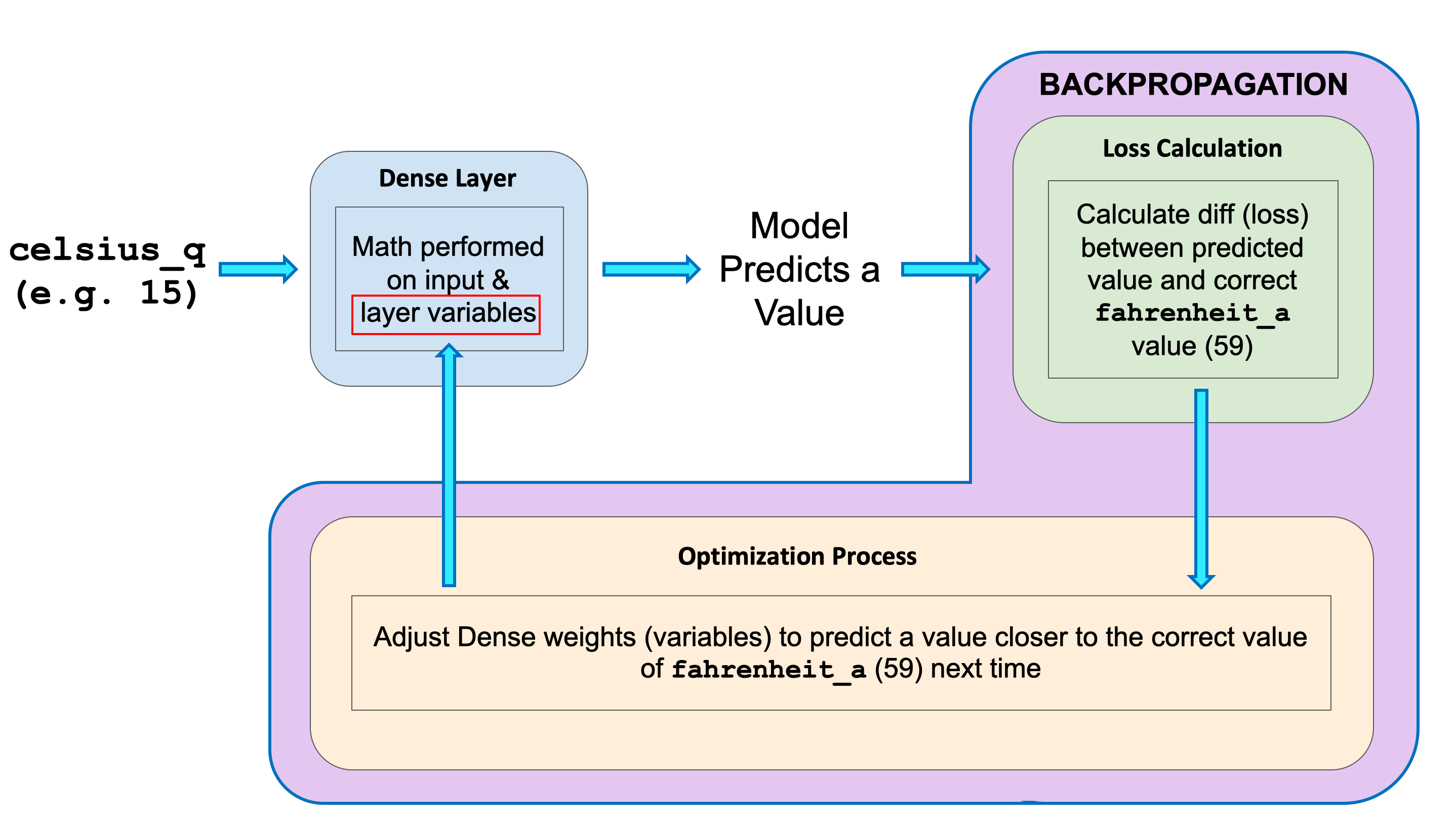
This optimization process is called Gradient Descent. The specific algorithm used to calculate the new value of each internal variable is specified by the optimizer parameter when calling model.compile(...). In this example we used the Adam optimizer.
Feature - The input(s) to our model.
Labels - The output our model predicts.
Examples - An input/output pair used for training. We break examples into two categories:
labeled examples: {features, label}: (x, y)
unlabeled examples: {features, ?}: (x, ?)
Model - A model defines the relationship between features and label.
Training - Training means creating or learning the model. That is, you show the model labeled examples and enable the model to gradually learn the relationships between features and label.
Inference - Inference means applying the trained model to unlabeled examples. That is, you use the trained model to make useful predictions (y').
Layer - A collection of nodes connected together within a neural network.
Weights and biases - The internal variables of model.
Loss - The discrepancy between the desired output and the actual output
Gradient Descent - An algorithm that changes the internal variables a bit at a time to gradually reduce the loss function.
Stochastic gradient descent (SGD) - uses only a single example (a batch size of 1) per iteration. Given enough iterations, SGD works but is very noisy.
Mini-batch stochastic gradient descent (mini-batch SGD) - is a compromise between full-batch iteration and SGD. A mini-batch is typically between 10 and 1,000 examples, chosen at random. Mini-batch SGD reduces the amount of noise in SGD but is still more efficient than full-batch.
Optimizer - A specific implementation of the gradient descent algorithm.
Learning rate - The “step size” for loss improvement during gradient descent.
Batch - The set of examples used during training in a single iteration.
Epoch - How many times this cycle should be run?
Forward pass - The computation of output values from input.
Backward pass (backpropagation) - The calculation of internal variable adjustments according to the optimizer algorithm, starting from the output layer and working back through each layer to the input.
Verbose - Argument controls how much output the method produces.
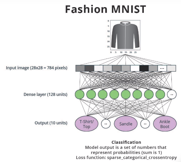
Flattening - The process of converting a 2d image into 1d vector.
Softmax - A function that provides probabilities for each possible output class.
📔 Notebook: Celsius_to_fahrenheit_with_FC
📔 Notebook: fashion_MNIST_with_FC
CNNs: Convolutional neural network. That is, a network which has at least one convolutional layer. A typical CNN also includes other types of layers, such as pooling layers and dense layers.
Convolution - The process of applying a kernel (filter) to an image.
Kernel / filter - A matrix which is smaller than the input, used to transform the input into chunks.
Padding - Adding pixels of some value, usually 0, around the input image.
Pooling - The process of reducing the size of an image through downsampling.There are several types of pooling layers. For example, average pooling converts many values into a single value by taking the average. However, maxpooling is the most common.
Maxpooling - A pooling process in which many values are converted into a single value by taking the maximum value from among them.
Stride - the number of pixels to slide the kernel (filter) across the image.
Downsampling - The act of reducing the size of an image.
Validation Set - We use a validation set to check how the model is doing during the training phase. Validation sets can be used to perform Early Stopping to prevent overfitting and can also be used to help us compare different models and choose the best one.
Resizing - When working with images of different sizes, you must resize all the images to the same size so that they can be fed into a CNN.
Color Images - Computers interpret color images as 3D arrays.
RGB Image - Color image composed of 3 color channels: Red, Green, and Blue.
Convolutions - When working with RGB images we convolve each color channel with its own convolutional filter. The result of each convolution is added up together with a bias value to get the convoluted output.
Max Pooling - When working with RGB images we perform max pooling on each color channel using the same window size and stride. Max pooling on each color channel is performed in the same way as with grayscale images, i.e. by selecting the max value in each window.
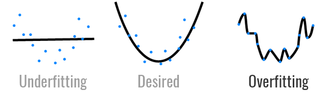
Overfitting refers to a model that fit the training data too well but cannot generalize well for new data.
Early Stopping - In this method, we track the loss on the validation set during the training phase and use it to determine when to stop training such that the model is accurate but not overfitting.
Image Augmentation - Artificially boosting the number of images in our training set by applying random image transformations to the existing images in the training set.
Dropout - Removing a random selection of a fixed number of neurons in a neural network during training.
📔 Notebook: fashion_MNIST_with_cnns
📔 Notebook: dogs_vs_cats_without_augmentation
📔 Notebook: dogs_vs_cats_with_augmentation
📔 Notebook: flowers_with_data_augmentation
Transfer Learning - A technique that reuses a model that was created by machine learning experts and that has already been trained on a large dataset. When performing transfer learning we must always change the last layer of the pre-trained model so that it has the same number of classes that we have in the dataset we are working with.
Freezing Parameters - Setting the variables of a pre-trained model to non-trainable. By freezing the parameters, we will ensure that only the variables of the last classification layer get trained, while the variables from the other layers of the pre-trained model are kept the same.
MobileNet - A state-of-the-art convolutional neural network developed by Google that uses a very efficient neural network architecture that minimizes the amount of memory and computational resources needed, while maintaining a high level of accuracy. MobileNet is ideal for mobile devices that have limited memory and computational resources.
📔 Notebook: Dog vs Cat and Transfer Learning
📔 Notebook: Flower and Transfer Learning
We can save trained model as HDF5 file, which is the format used by Keras. Then we can load the model. The model can be retrained and save.
This file includes:
- The model's architecture
- The model's weight values (which were learned during training)
- The model's training config (what you passed to `compile`), if any
- The optimizer and its state, if any (this enables you to restart
training where you left off)
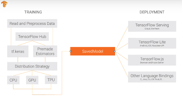
You can also export a whole model to the TensorFlow SavedModel format. SavedModel is a standalone serialization format for Tensorflow objects, supported by TensorFlow serving as well as TensorFlow implementations other than Python. A SavedModel contains a complete TensorFlow program, including weights and computation. It does not require the original model building code to run, which makes it useful for sharing or deploying (with TFLite, TensorFlow.js, TensorFlow Serving, or TFHub).
The SavedModel files that were created contain: * A TensorFlow checkpoint containing the model weights. * A SavedModel proto containing the underlying Tensorflow graph. Separate graphs are saved for prediction (serving), train, and evaluation. If the model wasn't compiled before, then only the inference graph gets exported. * The model's architecture config, if available.
Let's save our original `model` as a TensorFlow SavedModel. To do this we will use the `tf.saved_model.save()` function. This functions takes in the model we want to save and the path to the folder where we want to save our model. This function will create a folder where you will find an `assets` folder, a `variables` folder, and the `saved_model.pb` file.
📔 Notebook: Dog vs Cat and Saving and Loading Model
Each node in one layer is connected to each node in the previous layer.
ReLU function gives an output of 0 if the input is negative or zero, and if input is positive, then the output will be equal to the input.
ReLU gives the network the ability to solve nonlinear problems.
Make sure that your test set meets the following two conditions:
Mean square error (MSE)
The average squared loss per example over the whole dataset.
Time series is ordered sequence of value spread over time. Time series data is available in various place like stock price, weather forecast, demand trend, audio, GPS location log, brain wave etc.
Univariate time series is time series data with single value at each time-step.
Multivariate time series is time series with multiple value at each time-step.
Forecasting – process of predicting the future based on past and
present data. Use cases: Demand forecast, Weather forecast, …
Anomaly Detection – process of identifying unusual data points in dataset.
Use cases: Spam detection, fraud detection, …
Trend - A trend exists when there is a long-term increase or decrease in the data.
Seasonality - A seasonal pattern occurs when a time series is affected by seasonal factors such as the day of week.
Cyclic - A cycle occurs when the data exhibit rises and falls that are not of a fixed frequency.
Noise - Noise simply refers to random fluctuations of data.
Last period's actuals are used as this period's forecast. It is used as a based model for comparison.
Average value of moving window data used to smooth data.
Differencing – calculate different of each data point to
previous period for example -1 year to eliminate trend and seasonality.
(series(t) – series(t-365)
Linear relationship model with 1 dense layer.
RNN is a neural network which contains recurrent layers, that can sequentially
process a sequence of inputs. RNN contain memory cell which is used repeatedly
to compute the outputs. RNN expects 3D inputs: batch size, number of time-steps
and series dimension.
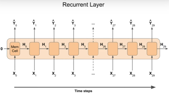
RNN > RNN > Dense
Sequent to Vector RNNs
Sequent to Sequent RNNs
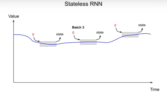
Stateless RNNs – NN resets state to zero at each iteration. Stateless
RNNs is simple to use but it cannot learn patterns longer than the length of the window.
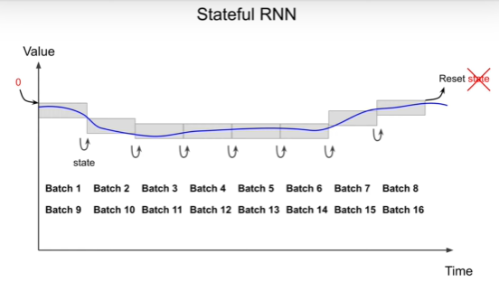
Stateful RNNs – NN which state is preserved for next training batch and
reset state to zero at the end of each epoch. It can learn from previous
state yet, it required more data preparation and take more time.
(used less compared to Stateless RNNs)
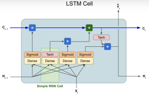
LSTM has short term and long time memory cell. LTSM call can detect patterns of over 100 time steps.
it is preferable to stack multiple convolutional layers with small kernel which increase performance and accuracy. Hyperparameter: Padding, Stride, No. of filter, Kernels
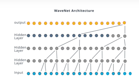
WaveNet is CNN model that has receptive field at different dilation rate to learn different time frame.
We use train and validation data to evaluate model and use full data including
test period for production deployment.
Fix partitioning - Split data into - Train, Validation, Test period
Roll-forward partitioning – Create series window of Train and Validation.
It required much more training time but it more mimic production condition.
| Metrics | Explaination |
|---|---|
| errors | forecast – actual |
| mse (mean square error) |
np.square(errors).mean() |
| rmse (root mean square error) |
pow(mse, 2) |
| mae (mean absolute error) |
np.abs(errors).mean() |
| mape (mean absolute percentage error) |
np.abs(errors/x_valid).mean() |
📔 Notebook: Time series patterns
📔 Notebook: Forecasing with Machine Learning
📔 Notebook: Forecasting with RNN
📔 Notebook: Forecasting wiht Stateful RNN
📔 Notebook: Forecasting wiht LSTM
📔 Notebook: Forecasting wiht CNN
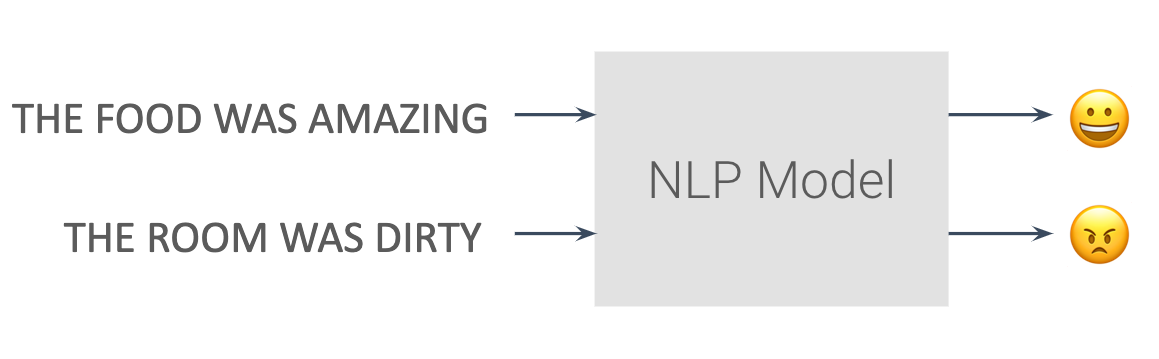
Natural Language Processing, or NLP for short, focuses on analyzing text and speech data. This can range from simple recognition (what words are in the given text/speech), to sentiment analysis (was a review positive or negative), and all the way to areas like text generation (creating novel song lyrics from scratch).
NLP got its start mostly on machine translation, where users often had to create strict, manual rules to go from one language to another. It has since morphed to be more machine learning-based, reliant on much larger datasets than the early methods were.
Tokenization
- Tokenizing
- Padding sequences
- OOV (Out of vocabulary words)
- Use real datasets
Embeddings
- Transform into Enbeddings
- Develop a Sentiment Model
- Visualize Embedding Space
- Tweak Hyperparameters
- Diagnose Sequence Issues
RNN
- Sequence Context
- RNN Architecture
- Usage of LSTMs
- LSTM vs Convolution vs GRU
Text Generation
- Text Generation Basics
- LSTMs for Text Generation
- Optimizing Text Generation
Neural networks utilize numbers as their inputs, so we need to convert our input text into numbers. Tokenization is the process of assigning numbers to our inputs, but there is more than one way to do this - should each letter have its own numerical token, each word, phrase, etc.
Tokenizing based on letters with our current neural networks doesn’t always work so well - anagrams, for instance, may be made up of the same letters but have vastly different meanings. So, in our case, we’ll start by tokenizing each individual word.
Tokenizer
With TensorFlow, this is done easily through use of a Tokenizer, found
within tf.keras.preprocessing.text. If you wanted only the first 10 most
common words, you could initialize it like so:
tokenizer = Tokenizer(num_words=10)
Fit on Texts
Then, to fit the tokenizer to your inputs (in the below case a list of
strings called sentences), you use .fit_on_texts():
tokenizer.fit_on_texts(sentences)
Text to Sequences
From there, you can use the tokenizer to convert sentences into tokenized
sequences:
tokenizer.texts_to_sequences(sentences)
Out of Vocabulary Words (OOV)
However, new sentences may have new words that the tokenizer was not fit
on. By default, the tokenizer will just ignore these words and not include
them in the tokenized sequences. However, you can also add an “out of
vocabulary”, or OOV, token to represent these words. This has to be
specified when originally creating the Tokenizer object.
tokenizer = Tokenizer(num_words=20, oov_token=’OOV’)
Viewing the Word Index
Lastly, if you want to see how the tokenizer has mapped numbers to words,
use the tokenizer.word_index property to see this mapping.
tokenizer = Tokenizer(num_words=20, oov_token=’OOV’)
📔 Notebook: NLP Turn words into Tokens
Even after converting sentences to numerical values, there’s still an issue of providing equal length inputs to our neural networks - not every sentence will be the same length! There’s two main ways you can process the input sentences to achieve this - padding the shorter sentences with zeroes, and truncating some of the longer sequences to be shorter. In fact, you’ll likely use some combination of these.
pad_sequences
With TensorFlow, the pad_sequences function from
tf.keras.preprocessing.sequence can be used for both of these tasks. Given
a list of sequences, you can specify a maxlen (where any sequences longer
than that will be cut shorter), as well as whether to pad and truncate
from either the beginning or ending, depending on pre or post settings for
the padding and truncating arguments. By default, padding and truncation
will happen from the beginning of the sequence, so set these to post if
you want it to occur at the end of the sequence. If you wanted to pad and
truncate from the beginning, you could use the following:
padded = pad_sequences(sequences, maxlen=10)
📔 Notebook: NLP prepare larger text corpus
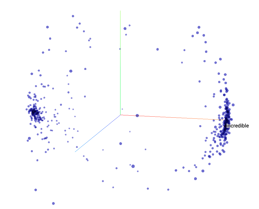
Embeddings are clusters of vectors in multi-dimensional space, where each vector represents a given word in those dimensions. While it’s difficult for us humans to think in many dimensions, luckily the TensorFlow Projector makes it fairly easy for us to view these clusters in a 3D projection (later Colabs will generate the necessary files for use with the projection tool). This can be very useful for sentiment analysis models, where you’d expect to see clusters around either more positive or more negative sentiment associated with each word.
To create our embeddings, we’ll first use an embeddings layer, called tf.keras.layers.Embedding. This takes three arguments: the size of the tokenized vocabulary, the number of embedding dimensions to use, as well as the input length (from when you standardized sequence length with padding and truncation).
The output of this layer needs to be reshaped to work with any fully-connected layers. You can do this with a pure Flatten layer, or use GlobalAveragePooling1D for a little additional computation that sometimes creates better results. In our case, we’re only looking at positive vs. negative sentiment, so only a single output node is needed (0 for negative, 1 for positive). You’ll be able to use a binary cross entropy loss function since the result is only binary classification.
They suggest that the final network does not use a sigmoid activation
layer when working with embeddings, especially when using just the two
classes like we are for sentiment analysis:
tf.keras.layers.Dense(1)
Additionally, they suggest instead of using the string
”binary_crossentropy” as the loss function, you use
tf.keras.losses.BinaryCrossentropy
(from_logits=True)
We’ve given you the code to create the files for input into the projector. This will download two files: 1) the vectors, and 2) the metadata. The projector will already come with a pre-loaded visualization, so you’ll need to use the “Load” button on the left and upload each of the two files.
In some cases, there may be a small difference in the number of tensors present in the vector file and the metadata file (usually with a message appearing after uploading the metadata); if this appears, wait for a few seconds for the error message to disappear, and then click outside the window. Typically, the visualization will still load just fine. Make sure to click the checkbox for “Sphereize data”, which will better show whether there is separation between positive and negative sentiment (or not).
There are a number of ways in which you might improve the sentiment analysis model we’ve built already:
Data and preprocessing-based approaches
- More data
- Adjusting vocabulary size (make sure to consider the overall size of the
corpus!)
- Adjusting sequence length (more or less padding or truncation)
- Whether to pad or truncate pre or post (usually less of an effect than
the others)
Model-based approaches
- Adjust the number of embedding dimensions
- Changing use of Flatten vs. GlobalAveragePooling1D
- Considering other layers like Dropout
- Adjusting the number of nodes in intermediate fully-connected layers
These are just some of the potential things you might tweak to better
predict sentiment from text.
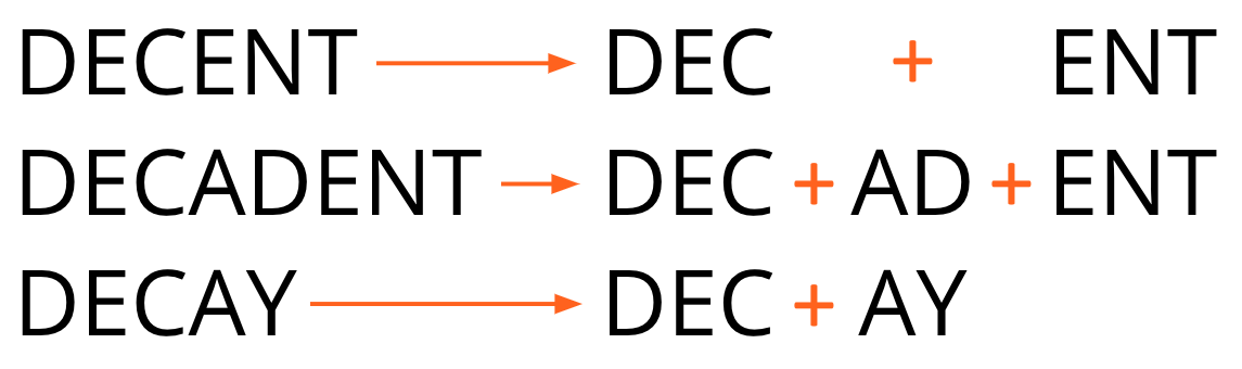
Subwords are another approach, where individual words are broken up into the more commonly appearing pieces of themselves. This helps avoid marking very rare words as OOV when you use only the most common words in a corpus.
recurrent neural networks will help understanding the full context of the sequence of words in an input.
There are a number of already created subwords datasets available online. If you check out the IMDB dataset on TFDS, for instance, by scrolling down you can see datasets with both 8,000 subwords as well as 32,000 subwords in a corpus (along with regular full-word datasets).
TensorFlow’s SubwordTextEncoder and its build_from_corpus function is used to create subwords from the reviews dataset we used previously.
🌐 A popular Github repo for NLP datasets
🌐 Google's public dataset search
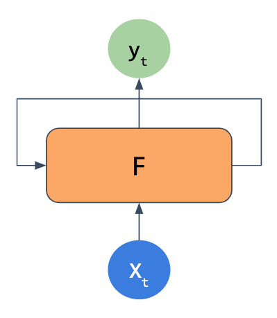
Recurrent Neural Networks (RNNs) still take in some input x and output some y, but they also feed some of the output of the network back into itself. This may be done over and over, so that with text input, the network has some memory of words that came much earlier in a sequence.
Simple RNNs are not always enough when working with text data. Longer sequences, such as a paragraph, often are difficult to handle, as the simple RNN structure loses information about previous inputs fairly quickly.
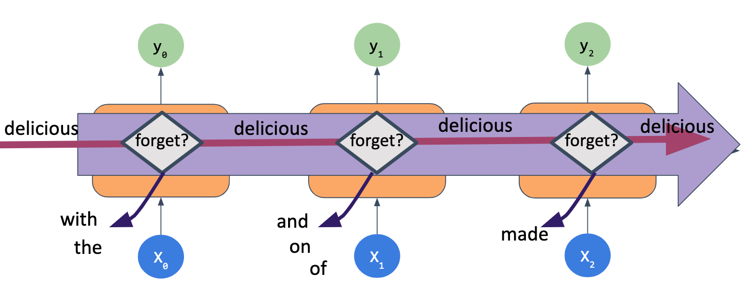
Long Short-Term Memory models, or LSTMs, help resolve this by keeping a “cell state” across time. These include a “forget gate”, where the cell can choose whether to keep or forget certain words to carry forward in the sequence. Another interesting aspect of LSTMs is that they can be bidirectional, meaning that information can be passed both forward (later in the text sequence) and backward (earlier in the text sequence).
The code for an LSTM layer itself is just the LSTM layer from tf.keras.layers, with the number of LSTM cells to use. However, this is typically wrapped within a Bidirectional layer to make use of passing information both forward and backward in the network, as we noted on the previous page.
tf.keras.layers.Bidirectional
(tf.keras.layers.LSTM(64))
One thing to note when using a Bidirectional layer is when you look at the model summary, if you put in 64 LSTM nodes, you will actually see a layer shape with 128 nodes (64x2).
No Need to Flatten
Unlike our more vanilla neural networks in the last lesson, you no longer
need to use Flatten or GlobalAveragePooling1D after the LSTM layer - the
LSTM can take the output of an Embedding layer and directly hook up to a
fully-connected Dense layer with its own output.
Doubling Up
You can also feed an LSTM layer into another LSTM layer. To do so, on top
of just stacking them in order when you create the model, you also need to
set return_sequences to True for the earlier LSTM layer - otherwise, as
noted above, the output will be ready for fully-connected layers and not
be in the sequence format the LSTM layer expects.
📔 Notebook: LSTMs with Subword
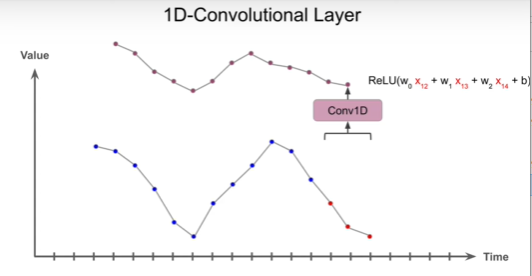
Convolutional Layers for Text
Just like you did with images, you can also use convolutional layers on
text, where the convolution occurs across a sequence of words instead of
across an image. To use a convolutional layer on text inputs, you can
place a Conv1D layer directly after the Embedding layer:
tf.keras.layers.Conv1D
(128, 5, activation=’relu’)
Note that you will need to use Flatten or GlobalAveragePooling1D on the output of this layer to connect to any fully-connected layers from there.
GRUs(Gated Recurrent Units)
Gated Recurrent Units, or GRUs, have “update” and “reset” gates. These
gates decide what to keep and what to throw away. They do not have a “cell
state” like LSTMs do. The code for these is very similar to an LSTM, where
the GRU layer is wrapped in a Bidirectional layer.
tf.keras.layers.Bidirectional
(tf.keras.layers.GRU(32))
An important item to note here is these performance differences (with perhaps the exception of training duration) will vary depending on the dataset and other changes to the model - you shouldn’t always assume one type of model will work better than another.
CNN
Utilizes “filters” that can slide over multiple words at a time and
extract features from those sequences of words. Can be used for purposes
other than a recurrent neural network.
GRU
Utilizes “update” and “reset” gates, where the “update” gate determines
updates to the existing stored knowledge, and the reset gate determines
how much to forget in the existing stored knowledge.
LSTM
Utilizes “forget” and “learn” gates that feed to “remember” and “use”
gates, where remembering is for further storage for the next input, and
using is for generating the current output.
📔 Notebook: NLP with multiple models comparison
🌐 Documentation for GRU layers in TensorFlow
🌐 Documentation for LSTM layers in TensorFlow
🌐 Documentation for 1D Convolutional layers in TensorFlow
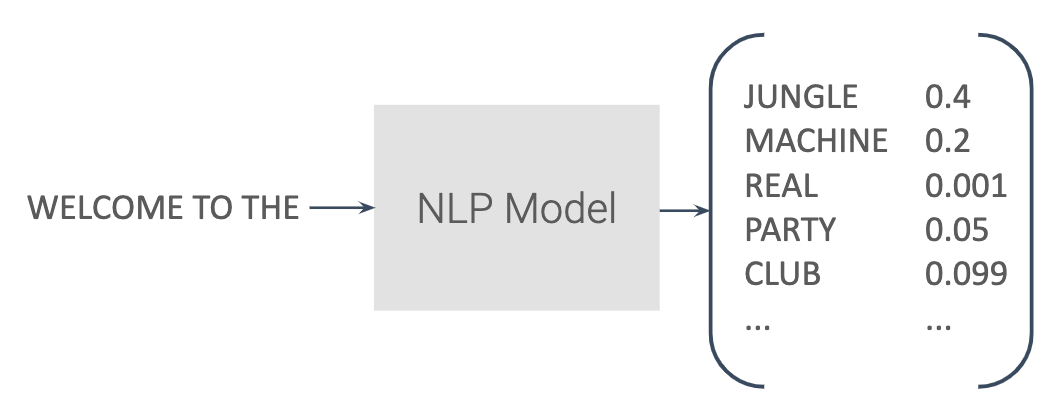
Text generation can be done through simply predicting the next most likely word, given an input sequence. This can be done over and over by feeding the original input sequence, plus the newly predicted end word, as the next input sequence to the model. As such, the full output generated from a very short original input can effectively go on however long you want it to be.
The only real change to the network here is the output layer will now be equivalent to a node per each possible new word to generate - so, if you have 1,000 possible words in your corpus, you’d have an output array of length 1,000. You’ll also need to change the loss function from binary cross-entropy to categorical cross entropy - before, we had only a 0 or 1 as output, now there are potentially thousands of output “classes” (each possible word).
There are hardly any differences in the model itself, other than changing the number of nodes in the output layer and changing the loss function. The more obvious changes come in working with the input and output data. The input data takes chunks of sequences and just splits off the final word as its label. So, if we had the sentence “I went to the beach with my dog”, and we had a max input length of five words, we’d get:
Input: I went to the beach
Label: with
Now, that’s not the only sequence that will come from the sentence! We would also get:
Input: went to the beach with
Label: my
And
Input: to the beach with my
Label: dog
That’s how the N-Grams used in the pre-processing work - a single input sequence might actually become a series of sequences and labels. With the output of the network, I’ll let you mostly investigate that code in the Colab on the next page, but the important thing there is that you can keep looping and creating more text by just appending the next word onto the previous input sequence.
📔 Notebook: NLP CNN song generation
There are a number of ways you might improve your text generation
models:
Using more data?
You’ll need to consider memory and output size constraints
- Also consider using only top-k most common words
- Know your data - songs have many more words than a Tweet
Keep tuning your model
- Add/subtract from layer sizes or embedding dimensions
Use np.random.choice with the probabilities for more variance in predicted
outputs
📔 Notebook: NLP optimizing song generation
🎓 Google Developers Certification
🎓 TensorFlow Developer Certificate
🎓 Course: Deeplearning.ai TensorFlow in Practice Specialization
🎓 Course: Deeplearning.ai TensorFlow in Practice Specialization
🎓 Course: Machine Learning Crash Course
🎓 Course: MIT Introdduction to Deep Learning
🌐 Github: Hands-on Machine Learning with Scikit-Learn, Keras and TensorFlow